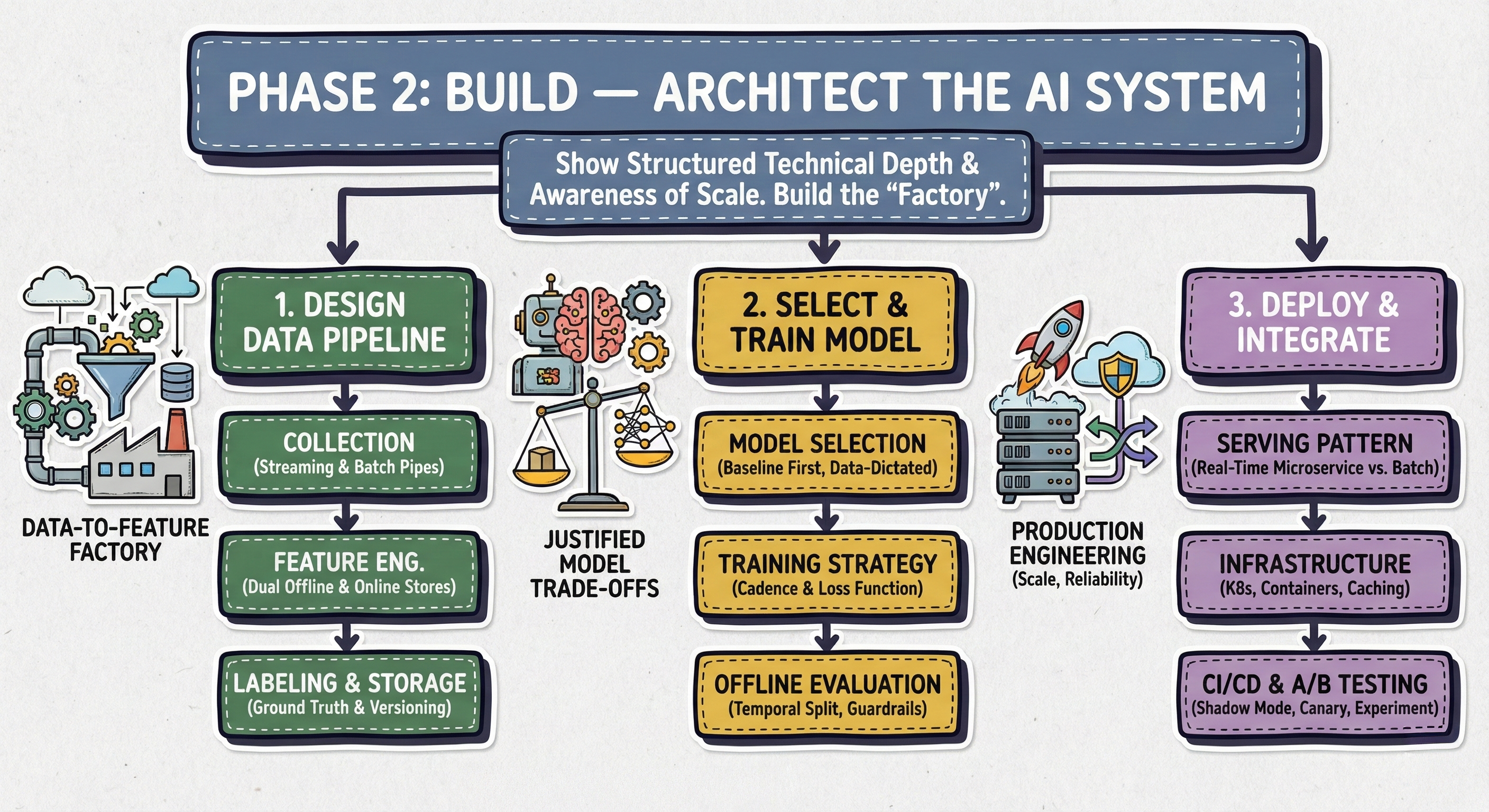
Phase 2 : BUILD - Architect the AI System

Phase 2: BUILD — Architect the AI System

Show structured technical depth and awareness of scale.

After acting as a "product-aware architect" in Phase 1, you now prove you are a world-class engineer who can handle the "how".

The main goal of this phase is to show structured technical depth and awareness of scale. You will move from a high-level sketch to architecting the actual "factory" that powers the AI system.

This phase consists of three steps:

1. Design the Data Pipeline: You'll design the reliable, scalable "data-to-feature" factory, often the most complex part of the system.

2. Select & Train the Model: You'll justify your model choice as a deliberate trade-off based on the project's specific constraints and objectives, not just choose the most complex model.

3. Deploy & Integrate: You'll detail the pure engineering required to get your model into production, focusing on scalability, reliability, and performance.

2.1. Design the Data Pipeline

Alright, this is it. If Phase 1 was about being a "product-aware architect," this step is where you prove you are a world-class data engineer. This is often the most complex part of any real-world AI system, and the one most likely to fail.

In Phase 1, you sketched the high-level blocks. Now, we're building the factory. Your goal here is to design the end-to-end "data-to-feature" factory that will reliably and scalably fuel your model. Your interviewer wants to see you handle scale, freshness, and complexity.

A junior engineer talks about a "data dump." A senior engineer designs a dual-pipeline system that separates offline batch processing from online stream processing. This is the single most important concept to demonstrate.

Let's break down how you'll explain this.

1. Data Collection & Ingestion (The "Front Door")

First, how does data get from the user's device into our system? You defined the sources in Step 2; now you name the "pipes."

• Streaming Data (For Freshness): "For a real-time system like a News Feed (Q1) or Fraud Detection (Q19), we can't wait hours for data. We need to capture user interactions (clicks, scrolls, transaction attempts) as they happen. This implies a message queue like Kafka or Kinesis. Our application servers will produce events (e.g., user_click_event) to a specific Kafka topic. This is our 'firehose' for all real-time data."

• Batch Data (For History): "We also have less time-sensitive, historical data. This includes user profile information, or large, daily logs. This data can be collected via a nightly batch ETL job and landed in our Data Lake (like S3 or Google Cloud Storage) or Data Warehouse (like BigQuery or Snowflake). This is our 'historical archive'."

2. Feature Engineering & Storage (The "Dual Pipeline")

This is the core of your design. Do not ever describe a single pipeline. You must separate the logic for training (offline) from the logic for serving (online). This separation solves for scale, cost, and freshness.

• The Offline Feature Pipeline:

  • Purpose: To create complex, historically-rich features for model training.

  • Process: "This is a daily batch job using a tool like Spark or dbt. It runs on our data warehouse, consuming all historical data—terabytes of it. It performs heavy-duty aggregations that are too slow for real-time."

  • Examples:

    • For News Feed (Q1): "user_7_day_click_rate_by_topic", "article_30_day_virality_score".

    • For Fraud Detection (Q19): "user_30_day_avg_transaction_value", "card_num_countries_used_in_last_90_days".

  • Storage: "The output is a massive feature table. These features are saved in our Offline Feature Store, which is typically our data warehouse or a Parquet file in S3."

• The Online Feature Pipeline:

  • Purpose: To create fresh, time-sensitive features for live inference.

  • Process: "This is a streaming application using Flink or Spark Streaming. It reads directly from Kafka. It computes features over short, sliding time windows (e.g., the last 1 minute, 10 minutes, 1 hour)."

  • Examples:

    • For News Feed (Q1): "user_num_clicks_in_last_5_minutes", "topics_user_is_browsing_right_now".

    • For Fraud Detection (Q19): "num_transactions_from_this_card_in_last_60_seconds", "is_this_transaction_value_5x_user's_1_hour_average?".

  • Storage: "These features must be retrieved in milliseconds. The output is written to a low-latency Online Feature Store, like Redis or Cassandra. This is the store our live prediction service will query."

• Why You Impress: By explaining this, you've shown you can provide both deep historical context (offline) and immediate user intent (online) to your model. You've also solved the #1 killer of ML systems: training-serving skew. You can state: "By using a shared feature transformation logic for both pipelines, and by using a Feature Store, we guarantee that the feature user_7_day_click_rate means the exact same thing in training as it does in serving."

3. Labeling Strategy (The "Ground Truth")

You have features, but what are you predicting? This links back to your objective (Step 1).

• Explicit Labels: "These are easy but rare. For a News Feed (Q1), this would be 'like', 'share', or 'hide'. For Airbnb (Q6), it's a 'booking'."

• Implicit Labels: "This is where we must be smarter. A 'click' is a weak positive signal. A 'click + dwell time > 30s' is a strong positive signal. A 'scroll-past' is an implicit negative. We'll need to define a 'success' event, like 'long click', to use as our positive label."

• Delayed Labels: "For Fraud (Q19) or Ads (Q21), the true label (e.g., 'chargeback' or 'purchase') might arrive days or weeks later. We must design our pipeline to handle this 'label delay' and stitch the label back to the features we had at the time of prediction."

4. Bias Handling & Data Versioning (The "Insurance Policy")

This is what separates a senior from a principal engineer. It's about reliability, reproducibility (getting the same results every time), and safety.

• Bias Handling: "Bias starts in the data. Before training, our pipeline must include jobs to analyze and mitigate bias.

  • Example for Job Recs (Q4): "We will audit our training data to ensure we have fair representation across demographics for 'qualified candidate' labels. If we find our data is skewed, we will use stratified sampling or oversampling (e.g., SMOTE for imbalanced classes) to create a more balanced training set."

• Data & Feature Versioning: "A model is 'code + data'. If our model performance suddenly drops, we must know if the data changed. Our pipeline will version its outputs. We won't just overwrite features; we'll save them as immutable, versioned datasets (e.g., partitioned by date in S3, or using a tool like DVC or LakeFS). This gives us perfect reproducibility: we can roll back a bad feature pipeline and retrain any old model on the exact data it was trained on."

By the time you're done, you haven't just "collected data." You've designed a reliable, scalable factory that is easy to check, versioned, and strong enough for a production environment. You've given your model a rock-solid foundation.

2.2. Select & Train the Model

Welcome to the "hero" step. This is what most people think the entire AI system design interview is about. But as you've just proven in Step 4, your model is nothing without a robust, scalable data pipeline. That hard data engineering work was the foundation; now, we get to build the skyscraper on top of it.

Your goal here is not to name the "latest, greatest, state-of-the-art model." That's a classic junior-engineer mistake. Your goal is to justify your model choice as a series of deliberate trade-offs based on everything you've already defined: your objective, your inputs, and your constraints.

Here's how you show you're a senior engineer who builds production systems, not a data scientist in an offline Kaggle competition.

1. Model Selection: A Justified Trade-off

You must demonstrate a "baseline-first" mentality and then justify your final choice based on the problem's data type and constraints.

• Always Start with a Simple Baseline:

  • "Before I build a complex deep learning model, my first step is to establish a strong, simple baseline. For a problem like Fraud Detection (Q19) or News Feed Ranking (Q1), this would be a Logistic Regression model on a small set of key, hand-crafted features."

  • Why? "This is critical for two reasons: First, it's fast to train, fast to serve, and highly interpretable. It gives us an immediate 'score to beat.' Second, we might find this simple model captures 90% of the business value for 1% of the engineering and compute cost, making it the right initial product, even if it's not the 'best' model."

• Justify Your "Production" Model Choice:

  Now, you select your primary model. Your choice must be dictated by your data.

  • For Tabular/Structured Data: (e.g., Fraud Detection (Q19), Ad Ranking (Q21), Job Matching (Q4) with engineered features)

    • "For this kind of structured, tabular data, Gradient Boosted Trees (GBCs)—specifically LightGBM or XGBoost—are the industry standard and my first choice. They are highly performant, handle sparse features and varying scales exceptionally well, and are far more interpretable than deep learning equivalents. They will almost certainly outperform our logistic regression baseline."

  • For Unstructured Data (Text/Image): (e.g., Content Moderation (Q14), Multi-Modal Search (Q9))

    • "Our input is raw text, so GBCs won't work. We need Deep Learning to create meaningful representations. I would choose a Transformer-based model. However, given our latency constraint (Step 2), a full-sized BERT or ViT is likely too slow for real-time inference. Therefore, I'd propose starting with a pre-trained, distilled model like DistilBERT or MobileNetV3. This gives us the power of transformers at a fraction of the inference cost. We can fine-tune this model on our internal, labeled data from Step 4."

• The Advanced Case: The Multi-Stage Architecture:

  • This is where you tie it all together. For any large-scale recommendation or search system (Q1-Q10), you must use the multi-stage architecture you defined in Step 3. This means you have two models to select.

  • 1. Retrieval Model (Candidate Generation): "For our News Feed (Q1), the retrieval model must scan billions of articles and pick ~1,000 in <30ms. The right choice here is a Two-Tower Model. One tower encodes the User (from user features) and the other tower encodes the Item (from article metadata). We train this with a contrastive loss to map similar user/items close in an embedding space. The magic is that we can pre-compute all item embeddings offline. At inference time, we just compute one user embedding and use an Approximate Nearest-Neighbor (ANN) search (like FAISS or ScaNN) to find the 1,000 closest items. This is extremely fast."

  • 2. Ranking Model: "Now that we have 1,000 candidates, we can afford a slower, more complex model. This is where our GBC (XGBoost) or a Wide-and-Deep DNN comes in. This model will use the full set of rich, real-time features from our Online Feature Store (Step 4)—features like 'user's clicks in the last 5 minutes'—that the retrieval model was too simple to handle. This model's job is to re-rank those 1,000 items to produce the final top 100 for the user."

2. Training Strategy & Evaluation

You've picked your model(s). Now, how do you build them?

• Training Cadence: "How often do we train? To start, I'd propose a daily batch retraining job. This job will use our Offline Feature Store, pulling, for example, the last 30 days of data. This balances model freshness (it learns from yesterday's data) with the stability and cost of training. We can version and save this model to our Model Registry."

• Loss Function (Matches the Objective!): "We must choose a loss function that directly optimizes our business metric from Step 1."

  • "For Fraud (Q19), we have a severe class imbalance. Using standard 'log-loss' will fail. We must use a weighted cross-entropy (to give more weight to the rare fraud class) or a focal loss to force the model to focus on hard-to-classify examples."

  • "For Ranking (Q1), we don't care about the exact score of one item; we care about the order of the whole list. Therefore, a point-wise loss (like MSE) is wrong. We must use a list-wise loss function like LambdaMART or Softmax Cross-Entropy, which directly optimizes for a ranking metric like NDCG."

• Offline Evaluation (The "Pre-flight Check"):

  • "We absolutely cannot evaluate our model on a simple random train-test split. Our data is time-sensitive."

  • "My evaluation strategy will be temporal. For our daily training job, we will train on 'Days 1-29' and test on 'Day 30' (the most recent day). This simulates a real production scenario of 'predicting the future' and is the only way to prevent data leakage and get a trustworthy offline metric."

  • "In this test, we will measure all our key metrics from Step 1: NDCG (for relevance), Precision/Recall (for classification), and, critically, our Guardrail Metrics (e.g., fairness metrics, bias audits) to ensure our new model is not just accurate but also safe."

You've now selected, justified, and laid out a complete training and evaluation plan. You've proven you're not just a model-user, but a model-builder who is obsessed with business value, constraints, and reliability.

2.3. Deploy & Integrate

You've done the "science." You've designed the data factory (Step 4) and you've trained a powerful, validated model (Step 5). Now comes the pure engineering. This is the step where your beautiful, high-performing model (which currently just exists in a notebook or a model registry) has to meet the high-scale, low-latency reality of production.

This is the "so what?" step. A model that can't be served reliably is just an academic exercise. Your interviewer is now switching hats. They are no longer a "data scientist." They are a "Site Reliability Engineer (SRE)" or a "Backend Systems Engineer." They are testing you on scalability, reliability, and performance.

Your goal is to explain how you'll get your model into production without breaking anything and how you'll prove it's working.

1. The First Big Decision: Batch vs. Real-Time Serving

Your first decision is to define your serving pattern, which you should have already hinted at in your earlier steps.

• Batch (Offline) Prediction:

  • What is it? This is a large-scale job, running on a schedule (e.g., daily), that pre-computes predictions for all (or many) users.

  • How it works: "For a system like a Spotify 'Discover Weekly' playlist or some job recommendations, we don't need real-time. I'd design a daily Spark job. It loads our model from the Model Registry, loads all user features from the Offline Feature Store, and generates recommendations for all active users. The results—a list of item_ids for each user_id—are then written to a simple key-value store, like Redis."

  • Integration: "When the user opens their app, the backend service doesn't call our model. It just does a fast key-value lookup in Redis. This is super-fast (sub-10ms), cheap, and highly reliable."

• Real-Time (Online) Inference:

  • What is it? This is what you'll need for most problems (Q1-Q19). It's a live, "always-on" service that generates predictions on demand.

  • How it works: "For our News Feed (Q1) or Fraud Detection (Q19), batch predictions are too stale. We must react to a user's current actions. Therefore, I will deploy our model as a real-time microservice."

  • Integration: "The application backend will make a synchronous API call (e.g., POST /getRankedFeed) to our service. Our service will, in real-time:

    1. Receive the user_id and context.

    2. Fetch fresh user features from the Online Feature Store (Redis) (Step 4).

    3. Execute our multi-stage model (Retrieval + Ranking) (Step 5).

    4. Return a ranked list, all within our <200ms latency budget (Step 2)."

2. Architecting the Real-Time Inference Service

Now, let's zoom in on that microservice.

• Infrastructure: "I would package our model artifact (e.g., the model.pkl file or TensorFlow graph) and our simple web server (e.g., FastAPI for Python, or gRPC for high-performance cross-service communication) into a Docker container. This container is our immutable, deployable unit."

• Orchestration: "We won't just deploy this container on one server. We will deploy it as a service on an orchestration platform like Kubernetes (K8s). This is necessary for large-scale systems. K8s gives us two critical features:

  1. Auto-scaling: It will automatically provision new containers as our request volume spikes.

  2. Fault Tolerance: If a container crashes, K8s will automatically restart it, ensuring high availability."

• Performance & Caching: "To meet our <200ms p99 latency, we need to be aggressive. First, the model itself must be optimized. If we're using a deep learning model, this means applying quantization (e.g., to FP16) or using a high-performance runtime like TensorRT. Second, we must cache. We'll use a cache like Redis at the API gateway level to store the final ranked list for active users for a short TTL (e.g., 1-2 minutes). If the same user pulls-to-refresh, we can serve directly from the cache, which bypasses our entire compute-heavy pipeline."

3. CI/CD for ML: Safe Deployment Strategy

You have a new model from Step 5. You have a live, running service from above. How do you deploy the new model without causing an outage?

• "We need a CI/CD pipeline for ML (MLOps). When a data scientist registers a new, validated model in our Model Registry, it automatically triggers this pipeline."

• Shadow Mode:

  • "First, the pipeline deploys the new model (Model B) to production in 'shadow mode.' Our live service (running Model A) will fork the production traffic. It sends the request to Model A (whose response goes to the user) and to Model B (whose response is logged but discarded)."

  • "This is our ultimate safety check. It lets us monitor Model B on live, real-world traffic with zero user impact. We can check for crashes, monitor p99 latency, and compare its prediction distribution to Model A's. This is how we catch the 'it-worked-in-the-notebook' bugs."

• Canary Rollout:

  • "Once Model B passes its shadow-mode checks, we begin a canary rollout. We configure our load balancer to send 1% of real user traffic to Model B. Those users see Model B's results."

  • "We now intensively monitor our Guardrail Metrics (from Step 1) on this 1% cohort. Does the *'Report Post'_ rate increase? Does latency spike? Does revenue drop? If all guardrails are healthy, we slowly ramp up: 5%, 20%, 50%, and finally 100%."

4. Online Evaluation: The A/B Test (The Only Ground Truth)

The canary rollout proved the model is safe. But is it better?

• "Offline metrics like NDCG (from Step 5) are just proxies. The only way to know if we achieved our primary business goal (e.g., 'increase D7 retention') is with a careful A/B test."

• "We will run a formal experiment: Group A (Control) sees Model A. Group B (Treatment) sees Model B. We will run this for at least two weeks to capture seasonality."

• "We will measure our primary, product-level metric from Step 1. Only if Model B shows a statistically significant win on our goal without harming our guardrails will it be promoted as the new, permanent production model. This is the final, definitive step of integration."